We’re going to give birth to a deep neural learning agent. OpenAI’s Gym is awesome, it’s the first Gym where I’m sure nobody will ask me like “Do you even lift bro?” (; So I even uploaded the agent, even though this is about sharing (which also helps me to learn) and not about competition.

The agent isn’t optimized for performance although it needs 51 steps, to solve the cart pole environment. If you want to, you can look at some stats and the evaluated performance here:

https://gym.openai.com/evaluations/eval_GFtDBmuyRjCzcAkBibwYWQ

If you haven’t heard about Deepmind’s Atari playing AI, which even earned them a Nature cover (Mnih et al., 2015), I strongly recommend starting with the video above, so you know what the hype’s all about. It’s a an easy, very entertaining 3 minute watch explaining why some people get so excited about the current advancements in reinforcement learning:

Recently Google’s AI think tank Deepmind revolutionized reinforcement learning by introducing Deep Q-Networks (DQN). DQN is a set of techniques which made it for the first time possible to really stabilize off-policy learning methods in conjunction with function approximation (especially by deep neural networks).

Reinforcement learning is a lot of fun and understanding the DQN algorithm is much easier than one might think. But sometimes getting from the math in a paper to an actual implementation still can be tricky. So I thought it could be helpful to share an easy implementation. I took some code of mine, stripped it down, removed all unnecessary clutter and used Keras to implement the networks to make it as easy as possible to understand the underlying algorithm.

Furthermore what Elon Musk’s no profit think tank OpenAI created with their Gym, a framework unifying the use of learning environments for AI agents, is the most addicting playground ever. The unified interface provided by Gym makes developing, testing and comparing learning algorithms so much easier and improves reproducibility to a great extend. So I hope I can also help by demonstrating how easy it is to interface with a Gym environment. The example we use is the cartpole task, a classic benchmark for control. Because the state representation is low dimensional, it’s no problem at all to train an agent even on a single CPU.

I extended DQN to double DQN because adding Hado van Hasselt’s Double-Q-Learning (Hasselt, 2010) to DQN helps to helps to stabilize the learning process even further and isn’t hardly any more difficult to implement (Van Hasselt, Guez, & Silver, 2015).

It might helpful to know the basics of RL. If you want to get started or need a refresher I recommend the following resources:

David Silver’s amazing lectures on RL at UCL.
Sutton and Barto’s classic book about the topic (Sutton & Barto, 1998) or even better the latest (free) draft of the upcoming 2nd edition.
Recently I began working on a code centric hands-on notebook explaining and visualizing tabular Q-learning. If you want to look into it or even give me some feedback, helping me to further improve it, this would be awesome:

Function approximation and Reinforcement Learning:

Avoiding Getting Killed by Blue Cars and Bowling Balls

For a long time most of reinforcement learning research took place on model problems with small discrete state spaces: 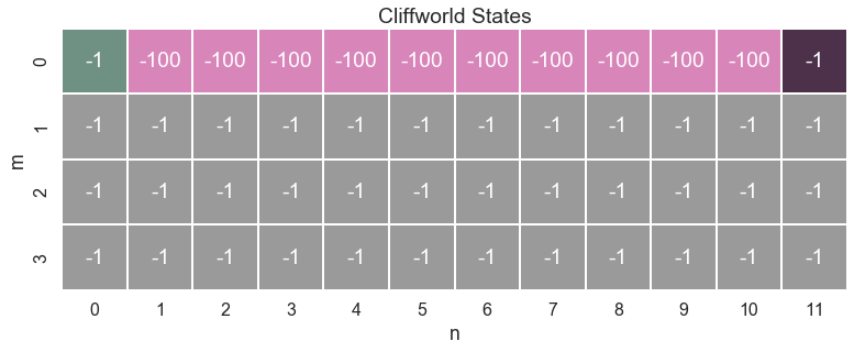Plot of Cliffworld a gridworld developed by Stutton and Barto These gridworlds are still a valuable tool for analyzing and understanding the properties of different algorithms. But one reason for the lack of success of RL outside such gridworlds was also what Richard Sutton calls the deadly triad.

Let’s look at the backup function for Q-learning:

$Q(s,a)\gets Q(s,a)+\alpha[r+\gamma \max_{a}Q(s',a)-Q(s,a)]$

The Q-function maps state-action pairs to a scalar value. For a small gridworld with $4 \times 12$ available states and 4 possible actions there are $4 \times 12 \times 4 = 512$ Q-value estimates needed to represent the Q-function. It’s easy to see, that the number of estimates will grow quickly for larger state and action spaces and that the simple tabular representation wouldn’t work at all for continuous state spaces. Moreover convergence to the true Q-values is only guaranteed if each state-action pair is visited a infinite number of times (Watkins & Dayan, 1992), so learning the Q-function of large state-action spaces is virtually impossible.

It’s easy to understand that this is a problem of almost all learning. If we get hit by a red car, why will we (hopefully) jump to the side the next time a car approaches us at high velocity even if it’s a blue car this time? And what about deciding whether to catch a spherical object or not? If we successfully caught a basketball, why won’t most people try the same thing with a bowling ball?

Because we never experience the exact same situation twice, we have to generalize from multiple past experiences to successfully evaluate new situations.

Running Into the Deadly Triad

The proven ability (imposing only some mild conditions) of neural networks to approximate arbitrary continuous functions by superposition the activation functions of its neurons (Csáji, 2001) makes it only a natural choice to use them to represent the Q-function. So the approximate Q-function

$Q(s,a) \approx Q(s,a, \mathbf{w})$

is now parameterized by the weights $\mathbf{w}$ of the neural network. But this naive approach will be highly unstable. Why’s that so? We’re encountering what Sutton calls the deadly triad:

Learning combining the following three conditions is always most likely to diverge:

off-policy learning, like it’s the case with Q-learning due to the $max$ operator in the Bellman update
scalable function approximation
bootstrapping, meaning estimating estimates from estimates, which is the main principle of Temporal-Difference learning methods

Even linear function approximation in seemingly very simple environments can lead to instable, diverging Q-functions. I strongly recommend taking a look at Baird’s counterexample (Baird & others, 1995). Leemond Baird constructed an example using the simplest MDP one could think of, where linear function approximation still needs to divergence of the Q-function.

DQN to the Rescue

Until the development of DQN it has impossible to stabilize learning under the conditions of the deadly triad. DQN provides a set of three methods to stabilize the learning process. The first one which is clipping the rewards to a fixed range, is pretty straight forward.

Clipping the TD-error to a fixed interval of $[-1, 1]$
Experience replay
Replacing one single network by the use of two separate networks, one online network and one target network

The first one is pretty straight forward. So let’s talk about experience replay and the target network.

Experience Replay or Flashbacks

Neural networks have been successfully used for supervised learning for years. So the main idea behind DQN is to find a way of brining training of the network in RL closer to the supervised setting. Experiences consisting of the tuple $(s, a, s', r)$ , state, action, nextstate, reward, are not directly used to update the Q-function. Instead they are stored in a replay memory of fixed size. The Q-function now is updated by sampling a random batch of memory tuples at each timestep from this memory. This has several advantages:

Now it is possible to use Mini-batch gradient descent to optimize the loss of the network, which reduces variance.
At each timestep it is now possible to learn from multiple samples not just from the recent transition.
Learning implies the assumption of the samples being i.i.d. Because the samples are generated by a sequence of subsequent steps by the agent, they violate this assumption. Decoupling generating samples from learning samples by using the memory as a proxy brings the distribution of samples used for learning closer to the i.i.d assumption.

Couldn’t resist to call this Flashback, it sounds so much cooler. Sorry (:

Using a fixed target network

Let’s look at the backup for the Q-function again:

$Q(s,a)\gets Q(s,a)+\alpha[r+\gamma \max_{a}Q(s',a)-Q(s,a)]$

Using a neural network, both the targets given by $\gamma \max_{a}Q(s',a, \mathbf{w})$ as well as the updated values $Q(s,a,\mathbf{w})$ depend on the weights $\mathbf{w}$ of the neural network. So a weight update that increases $Q(s,a,\mathbf{w})$ potentially also increases $\gamma \max_{a}Q(s',a, \mathbf{w})$ which could result in feedback. To address this issue two separate networks are used. The online network parametrized by $\mathbf{w^⁻}$ is used to generate the Q-values for epsilon greedy action selection. To compute the targets $Y_{DQN}=\gamma \max_{a}Q(s',a, \mathbf{w^⁻})$ a second network, the target network parametrized by $\mathbf{w^⁻}$ is used. At each timestep the weights of the online network are updated by optimizing the MSE loss function

$\mathcal{L}(w) = \mathbb{E}_{s,a,r,s'\sim \mathcal{D}}[(r+\gamma\max_{a}Q(s',a,\mathbf{w^{-}})-Q(s,a,\mathbf{w}))^{2}]$

via mini-batch gradient descent. The weights $\mathbf{w^⁻}$ of the target network are kept fixed and only periodically updated by copying the weights from the online network: $\mathbf{w^⁻}\gets \mathbf{w}$ This avoids destabilizing feedback loops in the update of the Q-function. Only after the weight updates DQN generated for a short time to the simple Q-learning case because $\mathbf{w^⁻}=\mathbf{w}$ , it’s practically the same as using a single network.

Tackling Value Overestimation by Extending DQN to Double DQN

To be honest, the cart-pole example we’re using here, won’t benefit much from extending DQN to Double DQN. This is due to the fact that overestimation bias increases with the number of possible actions (Van Hasselt, Guez, & Silver, 2015) and the classic cart-pole domain is a bang bang control problem (just discrete actions, “on or off”) with only 2 available actions. Nevertheless the code will way more stable in other environments. Because RL is general and not problem specific, you can use the same code for a wide variety of problems and when a convolution layer is added and the parameters are tuned it performs well on raw pixels. The benefits of Double DQN will also increase, when confronted with noisy environments and especially noisy reward signals. So adding double DQN right away is worth it. While the recent paper (Van Hasselt, Guez, & Silver, 2015) about double DQN is accessible if one invests a little time, the original paper by Hado van Hasselt introducing Double-Q-Learning is a really challenging read (Hasselt, 2010). I try to provide some intuition here but if you really want to get into the mathematics behind the overestimation bias I recommend the following steps:

Begin with Jensen’s Inequality. This video is a great starting point before looking at the proofs.
Read the passage on Double-Q-Learning in the draft version of Sutton and Barto’s book.
Read the Double DQN paper (Van Hasselt, Guez, & Silver, 2015)
Finally read Thrun and Schwartz’ paper about function approximation and overestimation biases in RL (Thrun & Schwartz, 1993) and Hado van Hasselt’s original paper introducing Double Q-learning.

Basically Q-learning uses $\mathbb{E}[\max_{a}Q(s',a)]$ to approximate $\max_{a}\mathbb{E}[Q(s',a)]$ , which is always less or equal. Using the max over all Q-values, we always select the one, with the highest probability of overestimation (when there’s noise or function approximation). It’s easy to understand that expectation of these estimates now has an upwards bias.

Double DQN decomposes the max operation for the target values into action selection and action evaluation. The targets are now

$Y_{DDQN}=r+\gamma Q(s', \mathop{\arg\,\max}\limits_a Q(s',a,\mathbf{w}), \mathbf{w^⁻})$

so the argmax of the Q-values of the online network for a particular state maps this state to an action, now the target network’s Q-value is a function of this state and the action selected by the online network.

Shut up and show me the code!

I sacrificed some DRYness and extendability of the code, to make the underlying algorithm as understandable as possible. To keep it simple I also sinned and used global variables for configuration to avoid bloated commandline parsing. If something isn’t clear, feel free to ask my anytime. Here I want to explain the parts I consider most important.

The whole code is consists of the following parts:

Experiment: Wrapper around the Gym environment. Also containing the control flow for conducting the whole training as well as the agent-environment loop.
Agent: Learning agent, containing the learning logic as well as an instance of NN and the ReplayMemory
NN: Wrapping the online network model as well as the target network model_t
ReplayMemory: Storing the experience tuples and providing randomly sampled experience batches
EpsilonUpdater: Leftover from my own code. Using the observer pattern, to control greediness of action selection. Kept it, because it makes it simple to extend for adaptive control of other parameters like the learning rate or target network update frequency.
Utils Just some functions for reshaping numpy arrays

I wrapped the Gym environment in an experiment object which holds the agent-environment loop and all runtime logic for training.

Experiment

The main part is the run_episode method, which also contains the agent-environment loop.

def run_episode(self, agent):
    self.reward = 0
    s = self.env.reset()
    done = False
    while not done:
        self.env.render()
        a = agent.act(s)
        s_, r, done, _ = self.env.step(a)
        agent.learn((s, a, s_, r, done))
        self.reward += r
        s = s_

The interface of a Gym environment is very simple and consists of just 3 methods:

 reset() # resets environment and returns the start state
 step() # takes action, returns newstate, reward and true of false for being terminal
 render () # renders environment

Agent

Exposes just two methods to interface with the experiment. I tried to resemble the classic agent-environment interface as close as possible.

act() # takes state, returns action
learn() # takes state, action, newstate, reward, done bool and computes back ops

The _make_batch() method queries the ReplayMemory() for a batch of random samples. It also computes the targets, so it holds all the relevant ingredients for DQN and double DQN.

def run_episode(self, agent):
    self.reward = 0
    s = self.env.reset()
    done = False
    while not done:
        self.env.render()
        a = agent.act(s)
        s_, r, done, _ = self.env.step(a)
        agent.learn((s, a, s_, r, done))
        self.reward += r
        s = s_

NN

The brain of the agent. I used $\tanh$ as activation function because I think that rectified linear units (ReLU) don’t add any value for such small networks and low dimensional inputs. Furthermore we need some sort of gradient clipping, if we use ReLUs, because even smaller learning rates can lead to dying ReLUs. If you want to learn from pixels, you have to change just a few things:

Add 2 or 3 convolution layers
Increase general network size and add regularization (start with dropout, if needed try L2-norm weight regularization next)
Tweak the learning rate, now you also could benefit from switching to ReLU activation functions
Add some gradient clipping, don’t be so hard on the poor ReLUs <3

Optimization wise we use simple stochastic gradient descent. I think it’s a good baseline. The input doesn’t contain any spacial structure, where we could profit from convolution, so we just use simple fully connected layer. In my experience really small and and shallow networks perform best on such small problems. For higher dimensional inputs, especially for learning from raw pixel input or something like that, I recommend to be quite generous with layer size and use regularization to deal with overfitting.

I left this check if the loss is NaN in the code. If using ReLUs you should notice if the die and you have to start over (:

def flashback(self):
    X, y = self._make_batch()
    self.loss = self.NN.train(X, y)
    if np.isnan(self.loss.history['loss']).any():
        print('Warning, loss is {}'.format(self.loss))
    pass

Of course this is the very least. I didn’t want to clutter the code with all the bookkeeping stuff but if you don’t want to be blind, you wanna also compute the max Q-values, the loss and the values of the weights over time. You can’t have too many plots. Ever! (:

ReplayMemory

I used a double-ended queue to implement the maximum memory capacity. If the memory is queried for a batch and the batch size exceeds the current number of stored samples in the memory the memory returns the maximum number of samples available.

class ReplayMemory:
    def __init__(self, capacity):
        self.samples = deque([], maxlen=capacity)

    def store(self, exp):
        self.samples.append(exp)
        pass

    def get_batch(self, n):
        n_samples = min(n, len(self.samples))
        samples = sample(self.samples, n_samples)
        return samples

This works nice but if we want to implement prioritized replay, we need to use a Tree structure, so we’re able to achieve $\mathcal{O}(n\log{}n)$ search complexity (best case). But for now we’re happy with our simple deque (:

EpsilonUpdater

The EpsilonUpdater uses a push-oriented observer pattern. It’s easy to add more observers, to control additional parameters like the learning rate or update frequency at runtime. You can also add more events.

class EpsilonUpdater:
    def __init__(self, agent):
        self.agent = agent

    def __call__(self, event):
        if event == 'step_done':
            self.epsilon_update()
            self.switch_learning()
        else:
            pass

    def epsilon_update(self):
        self.agent.epsilon = (
            self.agent.epsilon_min +
            (self.agent.epsilon_max - self.agent.epsilon_min) * exp(
                -self.agent.epsilon_decay * self.agent.step_count_total))
        pass

    def switch_learning(self):
        if self.agent.step_count_total >= self.agent.learning_start:
            self.agent.learning_switch = True
        pass

The observer are attached via the agent’s add_observer() method:

def add_observer(self, observer):
    self.observers.append(observer)
    pass

The agent can push events to the observers by calling them using their magic __call__ method, which takes a simple string as identification for different events.

def notify(self, event):
    for observer in self.observers:
        observer(event)
    pass

Poledancing

Here’s some video of our beauty:

Some performance stats can be found here: